I was tasked to build a sample inferencing machine model that would be able to process a sample array of inputs and infer based upon these inputs the identity of a sample given.
To begin I wanted to attempt to start this model from scratch on a T2 Micro AMI
Launch AMI: Deep Learning AMI (Amazon Linux 2) Version 38.0
$ sudo yum update

#I see an example folder, I try to run the program and get errors
ModuleNotFoundError: No module named 'keras'
Also tensorflow is missing

#Install Keras and tensorflow, tensorflow shows a memory error! I run the following
$pip3 install --no-cache-dir tensorflow
$pip3 install keras

#Check the Tensorflow version, run script
    {
    import tensorflow as tf
    print(tf.__version__)
    }

#Attempt to run example inferencing model: Receive error!
    [root@ip-10-0-0-229 keras]# python3 cifar10_resnet.py
    2021-01-14 17:34:18.423066: I tensorflow/stream_executor/platform/default/dso_loader.cc:49] Successfully opened dynamic library libcudart.so.11.0
    Downloading data from https://www.cs.toronto.edu/~kriz/cifar-10-python.tar.gz
    170500096/170498071 [==============================] - 4s 0us/step
    Traceback (most recent call last):
    File "cifar10_resnet.py", line 72, in <module>
        x_train = x_train.astype('float32') / 255
    !!!!!!MemoryError: Unable to allocate 586. MiB for an array with shape (50000, 32, 32, 3) and data type float32!!!!!
    [root@ip-10-0-0-229 keras]#
It was now obvious that a T2 micro was not sufficient to run the model, I upgraded the instance to a T2 Medium with 4GB of Ram
#We need a bigger instance! upgrade to t2 medium with 4GB RAM

#Running the example program I see the epoch was set to 200!, I will use the simple exmaple I have seen online and build it myself
Epoch 1/200<---------
Learning rate:  0.001
 197/1563 [==>...........................] - ETA: 6:18 - loss: 2.3908 - accuracy: 0.2446


#My tensorflow script

import tensorflow as tf
import matplotlib.pyplot as plt

mnist = tf.keras.datasets.mnist
(x_train, y_train), (x_text, y_test) = mnist.load_data() #data of hand written numbers

plt.imshow(x_train[0])
plt.show()
I wanted to get images to show, a visual representation would be more desirable, I have a powerful computer myself so I decided to use my own Python environment and host a Jupyter notebook locally
#I want to be able to see a plot, this CLI method wont show me any examples. we will revert to using a Jupyter notebook on my own PC

Running Python 3.8.6 64bit
1. Go to scripts folder for python: ~\AppData\Local\Programs\Python\Python38\Scripts
2. Open CMD here, and run the following
    pip install Jupyter
    pip install keras
    pip install tensorflow
    pip install matplotlib

3. Run the Jupyter server,
    > jupyter notebook
    A Browser opens, click new and select Python3


#Check version using this simple script
{
import tensorflow as tf
tf.__version__
}
#Output: '2.4.0'
The dataset imported in used hand drawn models, I followed a tutorial online and I learned that normalizing the data value scale would allow faster processing. The following code snippet was used on the x_train and x_test data.
x_train = tf.keras.utils.normalize(x_train, axis=1)
x_test = tf.keras.utils.normalize(x_test, axis=1)
Before normalization 
After normalization
The code for the rest of the inferencing model is separated into two sections, one is the learning section, other is the prediction section. The following code needed to be used to process the dataset
import tensorflow as tf
    mnist = tf.keras.datasets.mnist #import dataset of numbers that are handwritten 0-9
    (x_train, y_train), (x_test, y_test) = mnist.load_data()

#normalize datapoints to scale from 0 to 1
    x_train = tf.keras.utils.normalize(x_train, axis=1)
    x_test = tf.keras.utils.normalize(x_test, axis=1)

#building model
    model = tf.keras.models.Sequential()
    model.add(tf.keras.layers.Flatten()) #flattening layer
    model.add(tf.keras.layers.Dense(128, activation=tf.nn.relu)) #using 128 neurons in layer
    model.add(tf.keras.layers.Dense(128, activation=tf.nn.relu))
    model.add(tf.keras.layers.Dense(10, activation=tf.nn.softmax))

#parameters of training
#Adam optimization algorithm
#sparse_catagorical_crossentropy, produces a category index of the most likely matching category
    model.compile(optimizer='adam',
                loss='sparse_categorical_crossentropy',
                metrics=['accuracy'])

    model.fit(x_train, y_train, epochs=3)
The following output was generated after processing 3 Epochs:
Epoch 1/3
1875/1875 [==============================] - 2s 996us/step - loss: 0.4842 - accuracy: 0.8598
Epoch 2/3
1875/1875 [==============================] - 2s 965us/step - loss: 0.1158 - accuracy: 0.9657
Epoch 3/3
1875/1875 [==============================] - 2s 964us/step - loss: 0.0707 - accuracy: 0.9773
<tensorflow.python.keras.callbacks.History at 0x1feaf5b9d60>
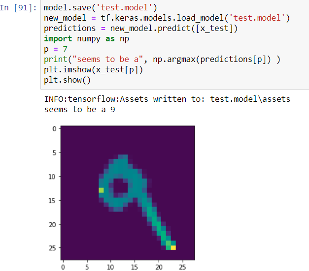
I then used the following script to test the model
#Testing the model 'p' is used as a prediction source
{model.save('test.model')
new_model = tf.keras.models.load_model('test.model')
predictions = new_model.predict([x_test])
import numpy as np
p = 7
print("seems to be a", np.argmax(predictions[p]) )
plt.imshow(x_test[p])
plt.show()
Some sample predictions can be seen below:


Testing Tensorflow with Fashion-MNIST samples

For this given tutorial I decided to try to run the program on my local computer, I skipped launching the REST server and wanted to run the program as is, the only change I needed to implement was to install a different version of grpcio, I used !pip install -Uq grpcio==1.32.0. The rest is straight foward and I will show my code below
#!/usr/bin/env python
# coding: utf-8

# In[1]:

import sys

# In[4]:

get_ipython().system('pip install -Uq grpcio==1.32.0')

# In[5]:

import tensorflow as tf
from tensorflow import keras

import numpy as np
import matplotlib.pyplot as plt
import os
import subprocess

print('TensorFlow version: {}'.format(tf.__version__))

# In[6]:

fashion_mnist = keras.datasets.fashion_mnist
(train_images, train_labels), (test_images, test_labels) = fashion_mnist.load_data()

# scale the values to 0.0 to 1.0
train_images = train_images / 255.0
test_images = test_images / 255.0

# reshape for feeding into the model
train_images = train_images.reshape(train_images.shape[0], 28, 28, 1)
test_images = test_images.reshape(test_images.shape[0], 28, 28, 1)

class_names = ['T-shirt/top', 'Trouser', 'Pullover', 'Dress', 'Coat',
               'Sandal', 'Shirt', 'Sneaker', 'Bag', 'Ankle boot']

print('\ntrain_images.shape: {}, of {}'.format(train_images.shape, train_images.dtype))
print('test_images.shape: {}, of {}'.format(test_images.shape, test_images.dtype))

# In[7]:

model = keras.Sequential([
  keras.layers.Conv2D(input_shape=(28,28,1), filters=8, kernel_size=3,
                      strides=2, activation='relu', name='Conv1'),
  keras.layers.Flatten(),
  keras.layers.Dense(10, activation=tf.nn.softmax, name='Softmax')
])
model.summary()

testing = False
epochs = 5

model.compile(optimizer='adam',
              loss='sparse_categorical_crossentropy',
              metrics=['accuracy'])
model.fit(train_images, train_labels, epochs=epochs)

test_loss, test_acc = model.evaluate(test_images, test_labels)
print('\nTest accuracy: {}'.format(test_acc))

# In[10]:

import tempfile

MODEL_DIR = tempfile.gettempdir()
version = 1
export_path = os.path.join(MODEL_DIR, str(version))
print('export_path = {}\n'.format(export_path))

tf.keras.models.save_model(
    model,
    export_path,
    overwrite=True,
    include_optimizer=True,
    save_format=None,
    signatures=None,
    options=None
)

print('\nSaved model:')

# In[36]:

def show(idx, title):
  plt.figure()
  plt.imshow(test_images[idx].reshape(28,28))
  plt.axis('off')
  plt.title('\n\n{}'.format(title), fontdict={'size': 16})


for p in range(4,9):
    show(p, 'An Example Image: {}'.format(class_names[test_labels[p]]))
I didn’t want to run the rest server, so I settled with showing my predictions as a range on the jupyter notebook:


